Example - GTC/OSIRIS
The spectrogrphy OSIRIS is one of the most used instrument on the Gran Telescopio Canarias (GTC). In this example, we wavelength calibration the R1000B HgAr arc.
Initialise the environment and the line list (see the other examples for using the NIST line list) for the data proecessing
from astropy.io import fits
import matplotlib.pyplot as plt
import numpy as np
from scipy.signal import find_peaks
from scipy.signal import resample

from rascal.calibrator import Calibrator
from rascal.util import refine_peaks

atlas = [
    3650.153, 4046.563, 4077.831, 4358.328, 5460.735, 5769.598, 5790.663,
    6682.960, 6752.834, 6871.289, 6965.431, 7030.251, 7067.218, 7147.042,
    7272.936, 7383.981, 7503.869, 7514.652, 7635.106, 7723.98
]
element = ['HgAr'] * len(atlas)
Load and inspect the arc image
data = fits.open('data_gtc_osiris/0002672523-20200911-OSIRIS-OsirisCalibrationLamp.fits')[1]

plt.figure(1, figsize=(16,5))
plt.imshow(np.log(data.data), aspect='auto', origin='lower')
plt.tight_layout()
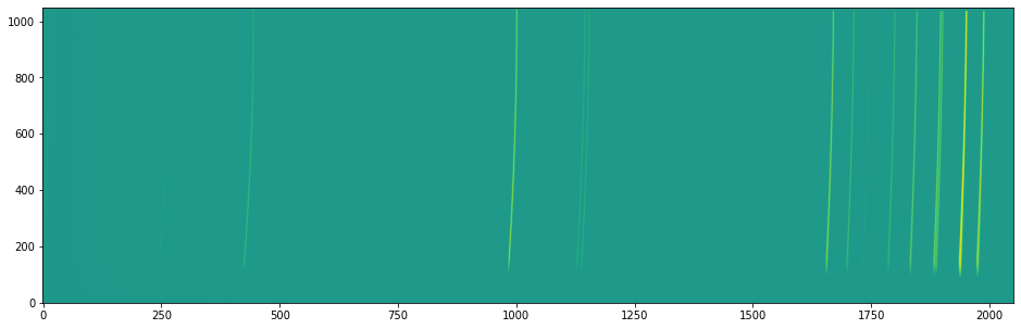
Normally you should be applying the trace from the spectral image onto the arc image, but in this example, we identify the arc lines in the middle of the frame.
spectrum = np.median(data.data.T[550:570], axis=0)

peaks, _ = find_peaks(spectrum, height=1250, prominence=20, distance=3, threshold=None)
peaks_refined = refine_peaks(spectrum, peaks, window_width=3)
Initialise the calibrator and set the properties. There are three sets of properties: (1) the calibrator properties who concerns the highest level setting - e.g. logging and plotting; (2) the Hough transform properties which set the constraints in which the trasnform is performed; (3) the RANSAC properties control the sampling conditions.
c.set_hough_properties(num_slopes=2000,
                       xbins=100,
                       ybins=100,
                       min_wavelength=3500.,
                       max_wavelength=8000.,
                       range_tolerance=500.,
                       linearity_tolerance=50)

c.load_user_atlas(elements=element,
                  wavelengths=atlas,
                  constrain_poly=True)

c.set_ransac_properties(sample_size=5,
                        top_n_candidate=5,
                        linear=True,
                        filter_close=True,
                        ransac_tolerance=5,
                        candidate_weighted=True,
                        hough_weight=1.0)

c.do_hough_transform()
The following INFO should be logged, where the first 3 lines are when the calibrator was initialised, and the last 3 lines are when the calibrator properties were set.
INFO:rascal.calibrator:num_pix is set to None.
INFO:rascal.calibrator:pixel_list is set to None.
INFO:rascal.calibrator:Plotting with matplotlib.
INFO:rascal.calibrator:num_pix is set to 2051.
INFO:rascal.calibrator:pixel_list is set to None.
INFO:rascal.calibrator:Plotting with matplotlib.
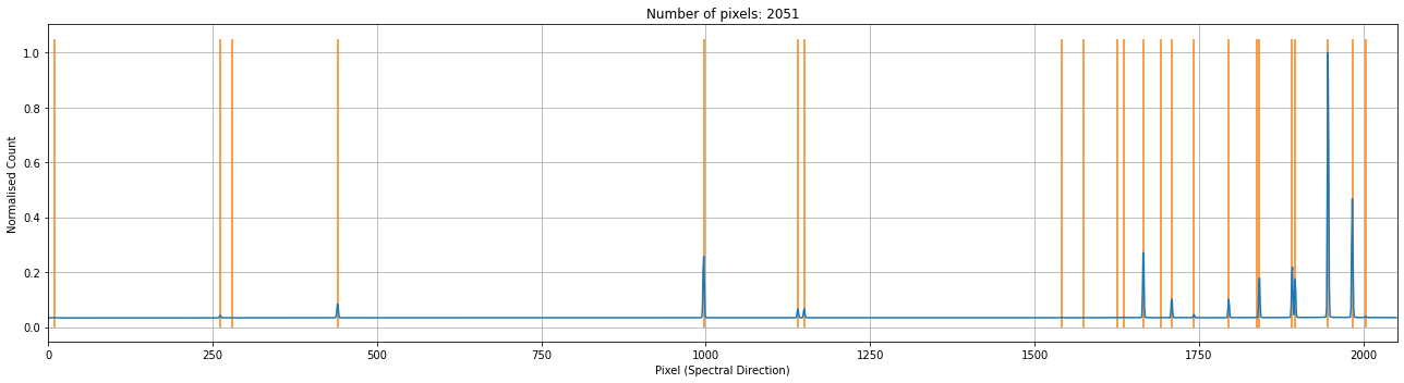
The extracted arc spectrum and the peaks identified can be plotted with the calibrator. Note that if only peaks are provided, only the orange lines will be plotted.
c.plot_arc()
Add the line list to the calibrator and perform the hough transform on the pixel-wavelength pairs that will be used by the RANSAC sampling and fitting.
c.load_user_atlas(elements=element,
                  wavelengths=atlas,
                  constrain_poly=True)
c.do_hough_transform()
Perform polynomial fit on samples drawn from RANSAC, the deafult option is to fit with polynomial function.
fit_coeff, rms, residual, peak_utilisation = c.fit(max_tries=200, fit_tolerance=10., fit_deg=4)

c.plot_fit(fit_coeff,
           plot_atlas=True,
           log_spectrum=False,
           tolerance=5.)
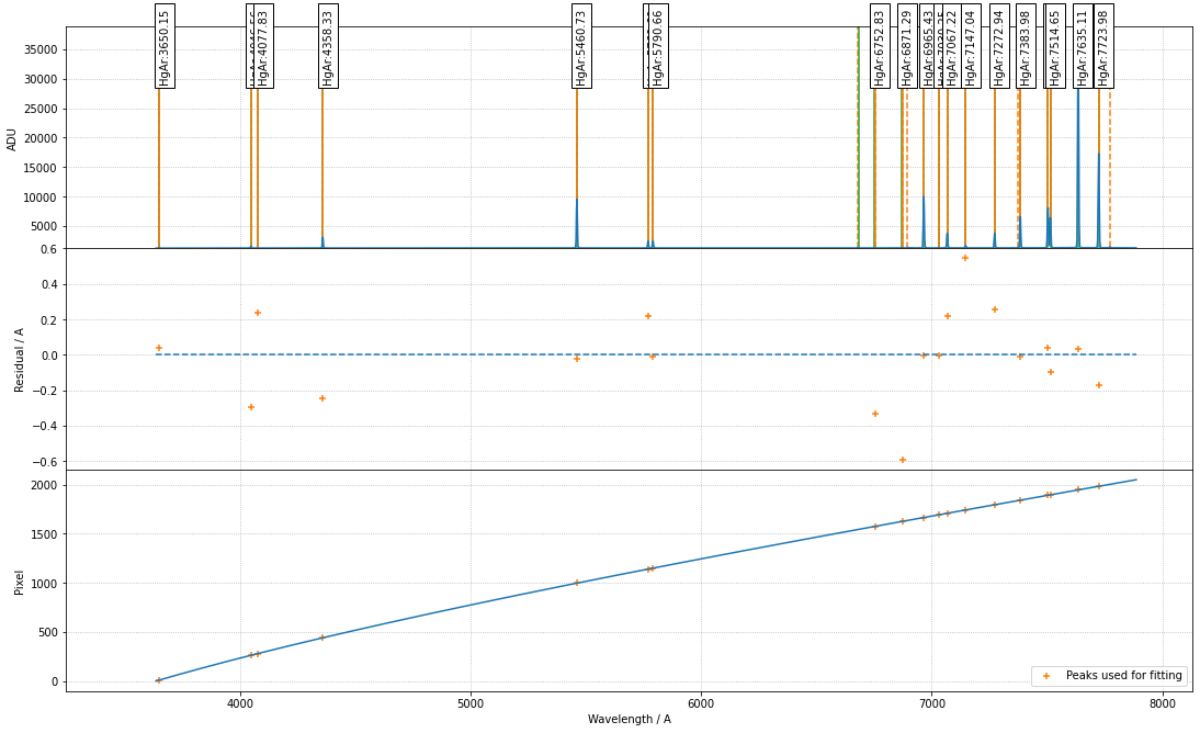
with some INFO output looking like this:
INFO:rascal.calibrator:Peak at: 3650.115449538473 A
INFO:rascal.calibrator:- matched to 3650.153 A
INFO:rascal.calibrator:Peak at: 4046.8620798203365 A
INFO:rascal.calibrator:- matched to 4046.563 A
INFO:rascal.calibrator:Peak at: 4077.595238720406 A
INFO:rascal.calibrator:- matched to 4077.831 A
INFO:rascal.calibrator:Peak at: 4358.576445488649 A
INFO:rascal.calibrator:- matched to 4358.328 A
INFO:rascal.calibrator:Peak at: 5460.7567985483165 A
INFO:rascal.calibrator:- matched to 5460.735 A
INFO:rascal.calibrator:Peak at: 5769.381771912414 A
INFO:rascal.calibrator:- matched to 5769.598 A
INFO:rascal.calibrator:Peak at: 5790.674908711722 A
INFO:rascal.calibrator:- matched to 5790.663 A
INFO:rascal.calibrator:Peak at: 6677.195577604758 A
INFO:rascal.calibrator:Peak at: 6753.169173651684 A
INFO:rascal.calibrator:- matched to 6752.834 A
INFO:rascal.calibrator:Peak at: 6871.881456822988 A
INFO:rascal.calibrator:- matched to 6871.289 A
INFO:rascal.calibrator:Peak at: 6894.527274171375 A
INFO:rascal.calibrator:Peak at: 6965.436232273663 A
INFO:rascal.calibrator:- matched to 6965.431 A
INFO:rascal.calibrator:Peak at: 7030.256183107306 A
INFO:rascal.calibrator:- matched to 7030.251 A
INFO:rascal.calibrator:Peak at: 7067.0001611640355 A
INFO:rascal.calibrator:- matched to 7067.218 A
INFO:rascal.calibrator:Peak at: 7146.4973429914635 A
INFO:rascal.calibrator:- matched to 7147.042 A
INFO:rascal.calibrator:Peak at: 7272.679474233918 A
INFO:rascal.calibrator:- matched to 7272.936 A
INFO:rascal.calibrator:Peak at: 7373.953964433149 A
INFO:rascal.calibrator:Peak at: 7383.992970996112 A
INFO:rascal.calibrator:- matched to 7383.981 A
INFO:rascal.calibrator:Peak at: 7503.831035910258 A
INFO:rascal.calibrator:- matched to 7503.869 A
INFO:rascal.calibrator:Peak at: 7514.750835501081 A
INFO:rascal.calibrator:- matched to 7514.652 A
INFO:rascal.calibrator:Peak at: 7635.073536260965 A
INFO:rascal.calibrator:- matched to 7635.106 A
INFO:rascal.calibrator:Peak at: 7724.151294456838 A
INFO:rascal.calibrator:- matched to 7723.98 A
INFO:rascal.calibrator:Peak at: 7772.136274228791 A
Quantify the quality of fit
print("RMS: {}".format(rms))
print("Stdev error: {} A".format(np.abs(residual).std()))
print("Peaks utilisation rate: {}%".format(peak_utilisation*100))
with these output
RMS: 0.263069686012686
Stdev error: 0.1791648865435056 A
Peaks utilisation rate: 80.0%
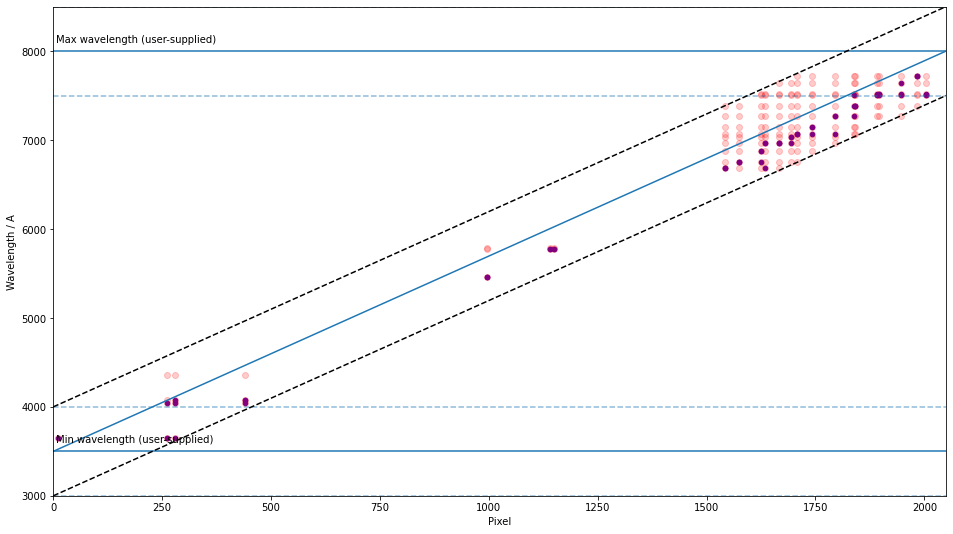
We can also inspect the search space in the Hough parameter-space where the samples were drawn by running:
c.plot_search_space()